Optical Flow

Goal

In this chapter,

• We will understand the concepts of optical flow and its estimation using Lucas-Kanade method.
• We will use functions like cv.calcOpticalFlowPyrLK() to track feature points in a video.
• We will create a dense optical flow field using the cv.calcOpticalFlowFarneback() function.

Optical Flow

Optical flow is the pattern of apparent motion of image objects between two consecutive frames caused by the movement of object or camera.

It assumes:

1. Pixel intensities do not change between consecutive frames.
2. Neighbouring pixels have similar motion (neighbourhood constraint).

Lucas-Kanade Method

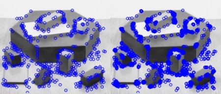
Lucas-Kanade method is a sparse optical flow method which assumes that the flow is essentially constant in a local neighbourhood. It solves the basic optical flow equations for all the pixels in that neighbourhood.

OpenCV provides a pyramid based version which handles large motions.

import numpy as np
import cv2 as cv

cap = cv.VideoCapture('slow.flv')

# params for ShiTomasi corner detection
feature_params = dict(maxCorners=100,
                      qualityLevel=0.3,
                      minDistance=7,
                      blockSize=7)

# Parameters for lucas kanade optical flow
lk_params = dict(winSize=(15, 15),
                 maxLevel=2,
                 criteria=(cv.TERM_CRITERIA_EPS | cv.TERM_CRITERIA_COUNT, 10, 0.03))

# Create some random colors
color = np.random.randint(0, 255, (100, 3))

# Take first frame and find corners in it
ret, old_frame = cap.read()
old_gray = cv.cvtColor(old_frame, cv.COLOR_BGR2GRAY)
p0 = cv.goodFeaturesToTrack(old_gray, mask=None, **feature_params)

# Create a mask image for drawing purposes
mask = np.zeros_like(old_frame)

while True:
    ret, frame = cap.read()
    if not ret:
        print('No frames grabbed!')
        break

    frame_gray = cv.cvtColor(frame, cv.COLOR_BGR2GRAY)

    # calculate optical flow
    p1, st, err = cv.calcOpticalFlowPyrLK(old_gray, frame_gray, p0, None, **lk_params)

    # Select good points
    if p1 is not None:
        good_new = p1[st == 1]
        good_old = p0[st == 1]

    # draw the tracks
    for i, (new, old) in enumerate(zip(good_new, good_old)):
        a, b = new.ravel().astype(int)
        c, d = old.ravel().astype(int)
        mask = cv.line(mask, (a, b), (c, d), color[i].tolist(), 2)
        frame = cv.circle(frame, (a, b), 5, color[i].tolist(), -1)

    img = cv.add(frame, mask)
    cv.imshow('frame', img)

    k = cv.waitKey(30) & 0xff
    if k == 27:
        break

    # Now update the previous frame and previous points
    old_gray = frame_gray.copy()
    p0 = good_new.reshape(-1, 1, 2)

cv.destroyAllWindows()

Dense Optical Flow

Lucas-Kanade method computes optical flow for a sparse feature set. OpenCV provides another algorithm to find the dense optical flow. It computes the optical flow for all the points in the frame based on Gunnar Farneback’s algorithm.

Below sample shows how to find the dense optical flow using above algorithm. We get a 2-channel array with optical flow vectors, (u,v). We find their magnitude and direction:

import numpy as np
import cv2 as cv

cap = cv.VideoCapture("vtest.avi")

ret, frame1 = cap.read()
prvs = cv.cvtColor(frame1, cv.COLOR_BGR2GRAY)
hsv = np.zeros_like(frame1)
hsv[..., 1] = 255

while True:
    ret, frame2 = cap.read()
    if not ret:
        print('No frames grabbed!')
        break

    next = cv.cvtColor(frame2, cv.COLOR_BGR2GRAY)
    flow = cv.calcOpticalFlowFarneback(prvs, next, None, 0.5, 3, 15, 3, 5, 1.2, 0)

    mag, ang = cv.cartToPolar(flow[..., 0], flow[..., 1])
    hsv[..., 0] = ang * 180 / np.pi / 2
    hsv[..., 2] = cv.normalize(mag, None, 0, 255, cv.NORM_MINMAX)

    bgr = cv.cvtColor(hsv, cv.COLOR_HSV2BGR)
    cv.imshow('frame2', bgr)

    k = cv.waitKey(30) & 0xff
    if k == 27:
        break

    prvs = next

cv.destroyAllWindows()

Source: OpenCV Python Tutorials — Original Documentation