Pose Estimation

Goal

In this section,

We will learn to exploit calib3d module to create some 3D effects in images.

Basics

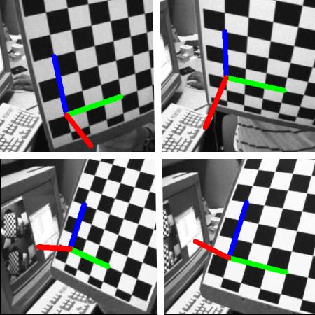
During the last session on camera calibration, you have found the camera matrix, distortion coefficients etc. Given a pattern image, we can utilize the above information to calculate its pose, or how the object is situated in space. For a planar object, we can assume Z=0.

Our problem is, we want to draw our 3D coordinate axis (X, Y, Z axes) on our chessboard’s first corner. X axis in blue color, Y axis in green color and Z axis in red color.

First, let’s load the camera matrix and distortion coefficients from the previous calibration result:

import numpy as np
import cv2 as cv
import glob

# Load previously saved data
with np.load('B.npz') as X:
    mtx, dist, _, _ = [X[i] for i in ('mtx', 'dist', 'rvecs', 'tvecs')]

Now let’s create a function, draw which takes the corners in the chessboard and axis points to draw a 3D axis:

def draw(img, corners, imgpts):
    corner = tuple(corners[0].ravel().astype("int32"))
    imgpts = imgpts.astype("int32")
    img = cv.line(img, corner, tuple(imgpts[0].ravel()), (255, 0, 0), 5)
    img = cv.line(img, corner, tuple(imgpts[1].ravel()), (0, 255, 0), 5)
    img = cv.line(img, corner, tuple(imgpts[2].ravel()), (0, 0, 255), 5)
    return img

Then we create termination criteria, object points and axis points. Axis points are points in 3D space for drawing the axis. We draw axis of length 3. X axis is drawn from (0,0,0) to (3,0,0), Z axis from (0,0,0) to (0,0,-3):

criteria = (cv.TERM_CRITERIA_EPS + cv.TERM_CRITERIA_MAX_ITER, 30, 0.001)
objp = np.zeros((6 * 7, 3), np.float32)
objp[:, :2] = np.mgrid[0:7, 0:6].T.reshape(-1, 2)

axis = np.float32([[3, 0, 0], [0, 3, 0], [0, 0, -3]]).reshape(-1, 3)

for fname in glob.glob('left*.jpg'):
    img = cv.imread(fname)
    gray = cv.cvtColor(img, cv.COLOR_BGR2GRAY)
    ret, corners = cv.findChessboardCorners(gray, (7, 6), None)

    if ret == True:
        corners2 = cv.cornerSubPix(gray, corners, (11, 11), (-1, -1), criteria)

        # Find the rotation and translation vectors.
        ret, rvecs, tvecs = cv.solvePnP(objp, corners2, mtx, dist)

        # project 3D points to image plane
        imgpts, jac = cv.projectPoints(axis, rvecs, tvecs, mtx, dist)

        img = draw(img, corners2, imgpts)
        cv.imshow('img', img)
        k = cv.waitKey(0) & 0xFF
        if k == ord('s'):
            cv.imwrite(fname[:6] + '.png', img)

cv.destroyAllWindows()

See some results below. Notice that each axis is 3 squares long:

3D axis pose estimation

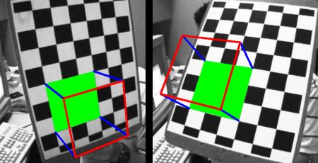
Render a Cube

If you want to draw a cube, modify the draw() function and axis points as follows:

def draw(img, corners, imgpts):
    imgpts = np.int32(imgpts).reshape(-1, 2)

    # draw ground floor in green
    img = cv.drawContours(img, [imgpts[:4]], -1, (0, 255, 0), -3)

    # draw pillars in blue color
    for i, j in zip(range(4), range(4, 8)):
        img = cv.line(img, tuple(imgpts[i]), tuple(imgpts[j]), (255), 3)

    # draw top layer in red color
    img = cv.drawContours(img, [imgpts[4:]], -1, (0, 0, 255), 3)

    return img

axis = np.float32([[0, 0, 0], [0, 3, 0], [3, 3, 0], [3, 0, 0],
                   [0, 0, -3], [0, 3, -3], [3, 3, -3], [3, 0, -3]])