· Hakan Çelik · OpenCV / Image Processing · 5 dk okuma
Image Thresholding

Image Thresholding
Image Thresholding
Goals
- In this article we will learn simple thresholding ( thresholding ), adaptive thresholding, and Otsu’s thresholding
- And we will learn these functions: cv2.threshold, cv2.adaptiveThreshold
Simple Thresholding
The problem is straightforward here. For every pixel, the same threshold value is applied. If the pixel value is greater than the threshold value, it is assigned one value (may be white), else it is assigned another value (may be black). The function used is cv2.threshold(). The first argument is the source image, which should be a grayscale image. The second argument is the threshold value used to classify the pixel values. The third argument is the maxVal which represents the value to be given if pixel value is greater than (sometimes less than) the threshold value. OpenCV provides different types of thresholding and it is determined by the fourth parameter of the function. These types are;
cv2.THRESH_BINARYcv2.THRESH_BINARY_INVcv2.THRESH_TRUNCcv2.THRESH_TOZEROcv2.THRESH_TOZERO_INV
Two outputs are obtained. The first is a retval which will be explained later. The second output is our thresholded image.
Code:
import cv2
import numpy as np
from matplotlib import pyplot as plt
img = cv2.imread('gradient.png',0) # we read the image, this is a
# grayscale image
# using all types to
# threshold the grayscale image
ret,thresh1 = cv2.threshold(img,127,255,cv2.THRESH_BINARY)
ret,thresh2 = cv2.threshold(img,127,255,cv2.THRESH_BINARY_INV)
ret,thresh3 = cv2.threshold(img,127,255,cv2.THRESH_TRUNC)
ret,thresh4 = cv2.threshold(img,127,255,cv2.THRESH_TOZERO)
ret,thresh5 = cv2.threshold(img,127,255,cv2.THRESH_TOZERO_INV)
titles = ['Original Image','BINARY','BINARY_INV','TRUNC','TOZERO','TOZERO_INV'] # defining a list and assigning the thresholded images and their names to two separate lists
images = [img, thresh1, thresh2, thresh3, thresh4, thresh5]
for i in range(6): # using a for loop to output the original and modified images to screen
    plt.subplot(2,3,i+1),plt.imshow(images[i],'gray')
    plt.title(titles[i])
    plt.xticks([]),plt.yticks([])
plt.show()
Note: We used
plt.subplot()function to plot multiple images. Please check out Matplotlib docs for more details.
The output of these codes gives an output like this.
Adaptive Thresholding
In the previous section, we used a global value as threshold value. But this might not be good in all cases where image has different lighting conditions in different areas. In that case, we go for adaptive thresholding. In this, the algorithm calculates the threshold for a small region of the image. So we get different thresholds for different regions of the same image and it gives us better results for images with varying illumination.
It has three ‘special’ input params and only one output argument.
Adaptive Method - It decides how thresholding value is calculated.
cv2.ADAPTIVE_THRESH_MEAN_C: threshold value is the mean of neighbourhood area.cv2.ADAPTIVE_THRESH_GAUSSIAN_C: threshold value is the weighted sum of neighbourhood values where weights are a Gaussian window.
Block Size - It decides the size of neighbourhood area.
C - It is just a constant which is subtracted from the mean or weighted mean calculated. The following code compares global thresholding and adaptive thresholding for an image with varying illumination:
import cv2
import numpy as np
from matplotlib import pyplot as plt
img = cv2.imread('dave.jpg',0)
img = cv2.medianBlur(img,5)
ret,th1 = cv2.threshold(img,127,255,cv2.THRESH_BINARY)
th2 = cv2.adaptiveThreshold(img,255,cv2.ADAPTIVE_THRESH_MEAN_C,\
            cv2.THRESH_BINARY,11,2)
th3 = cv2.adaptiveThreshold(img,255,cv2.ADAPTIVE_THRESH_GAUSSIAN_C,\
            cv2.THRESH_BINARY,11,2)
titles = ['Original Image', 'Global Thresholding (v = 127)',
            'Adaptive Mean Thresholding', 'Adaptive Gaussian Thresholding']
images = [img, th1, th2, th3]
for i in range(4):
    plt.subplot(2,2,i+1),plt.imshow(images[i],'gray')
    plt.title(titles[i])
    plt.xticks([]),plt.yticks([])
plt.show()
result

Otsu’s Binarization
In the first section, we mentioned that there is a second parameter retVal. Its use comes when we go for Otsu’s Binarization. So what does it do?
In global thresholding, we used an arbitrary value for threshold value, right? How do we know whether a value we selected is good or not? Answer is, trial and error method. But consider a bimodal image (In simple words, bimodal image is an image whose histogram has two peaks). For that image, we can approximately take a value in the middle of those peaks as threshold value, right? That is what Otsu binarization does. So in simple words, it automatically calculates a threshold value from image histogram for a bimodal image. (For images which are not bimodal, binarization won’t be accurate.)
For this, cv2.threshold() function is used, but pass an extra flag cv2.THRESH_OTSU. For threshold value, simply pass zero. Then the algorithm finds the optimal threshold value and returns it as the second output, retVal. If Otsu thresholding is not used, retVal is same as the threshold value you used.
Check out the example below. The input image is a noisy image. In the first case, I applied global thresholding for a value of 127. In the second case, I applied Otsu’s thresholding directly. In the third case, I filtered the image with a 5x5 Gaussian kernel to remove the noise, then applied Otsu thresholding. See how noise filtering improves the result.
import cv2
import numpy as np
from matplotlib import pyplot as plt
img = cv2.imread('noisy2.png',0)
# global thresholding
ret1,th1 = cv2.threshold(img,127,255,cv2.THRESH_BINARY)
# Otsu's thresholding
ret2,th2 = cv2.threshold(img,0,255,cv2.THRESH_BINARY+cv2.THRESH_OTSU)
# Otsu's thresholding after Gaussian filtering
blur = cv2.GaussianBlur(img,(5,5),0)
ret3,th3 = cv2.threshold(blur,0,255,cv2.THRESH_BINARY+cv2.THRESH_OTSU)
# plot all the images and their histograms
images = [img, 0, th1,
          img, 0, th2,
          blur, 0, th3]
titles = ['Original Noisy Image','Histogram','Global Thresholding (v=127)',
          'Original Noisy Image','Histogram',"Otsu's Thresholding",
          'Gaussian filtered Image','Histogram',"Otsu's Thresholding"]
for i in range(3):
    plt.subplot(3,3,i*3+1),plt.imshow(images[i*3],'gray')
    plt.title(titles[i*3]), plt.xticks([]), plt.yticks([])
    plt.subplot(3,3,i*3+2),plt.hist(images[i*3].ravel(),256)
    plt.title(titles[i*3+1]), plt.xticks([]), plt.yticks([])
    plt.subplot(3,3,i*3+3),plt.imshow(images[i*3+2],'gray')
    plt.title(titles[i*3+2]), plt.xticks([]), plt.yticks([])
plt.show()