Contour Features

Goals

In this article, we will learn:

To find the different features of contours, like area, perimeter, centroid, bounding box etc
You will see plenty of functions related to contours.

1. Moments

Image moments help you to calculate some features like center of mass of the object, area of the object etc.

The function cv2.moments() gives a dictionary of all moment values calculated:

import numpy as np
import cv2 as cv

img = cv.imread('star.jpg', cv.IMREAD_GRAYSCALE)
assert img is not None, "file could not be read, check with os.path.exists()"
ret, thresh = cv.threshold(img, 127, 255, 0)
contours, hierarchy = cv.findContours(thresh, 1, 2)

cnt = contours[0]
M = cv.moments(cnt)
print(M)

From this moments, you can extract useful data like area, centroid etc. Centroid is given by the relations Cx = M10/M00 and Cy = M01/M00:

cx = int(M['m10'] / M['m00'])
cy = int(M['m01'] / M['m00'])

2. Contour Area

Contour area is given by the function cv2.contourArea() or from moments, M['m00']:

area = cv.contourArea(cnt)

3. Contour Perimeter

It is also called arc length. It can be found out using cv2.arcLength() function. Second argument specify whether shape is a closed contour (if passed True), or just a curve:

perimeter = cv.arcLength(cnt, True)

4. Contour Approximation

It approximates a contour shape to another shape with less number of vertices depending upon the precision we specify. It is an implementation of Douglas-Peucker algorithm.

In this, second argument is called epsilon, which is maximum distance from contour to approximated contour. It is an accuracy parameter:

epsilon = 0.1 * cv.arcLength(cnt, True)
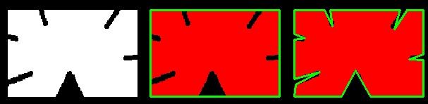
approx = cv.approxPolyDP(cnt, epsilon, True)

Below, in second image, green line shows the approximated curve for epsilon = 10% of arc length. Third image shows the same for epsilon = 1% of the arc length:

Contour approximation

5. Convex Hull

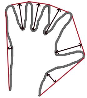
Convex Hull will look similar to contour approximation, but it is not the same. Here, cv2.convexHull() function checks a curve for convexity defects and corrects it. Generally speaking, convex curves are the curves which are always bulged out, or at-least flat. And if it is bulged inside, it is called convexity defects. For example, check the below image of hand. Red line shows the convex hull of hand:

Convex hull

Syntax:

hull = cv.convexHull(points[, hull[, clockwise[, returnPoints]]])

Arguments details:

points: the contours we pass into.
hull: the output, normally we avoid it.
clockwise: Orientation flag. If it is True, the output convex hull is oriented clockwise. Otherwise, it is oriented counter-clockwise.
returnPoints: By default, True. Then it returns the coordinates of the hull points. If False, it returns the indices of contour points corresponding to the hull points.

So to get a convex hull as in above image, following is sufficient:

hull = cv.convexHull(cnt)

6. Checking Convexity

There is a function to check if a curve is convex or not, cv2.isContourConvex(). It just returns True or False:

k = cv.isContourConvex(cnt)

7. Bounding Rectangle

There are two types of bounding rectangles.

7a. Straight Bounding Rectangle

It is a straight rectangle, it doesn’t consider the rotation of the object. It is found by the function cv2.boundingRect():

x, y, w, h = cv.boundingRect(cnt)
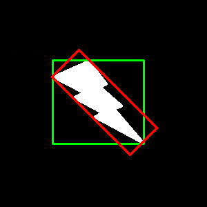
cv.rectangle(img, (x, y), (x + w, y + h), (0, 255, 0), 2)

7b. Rotated Rectangle

Here, bounding rectangle is drawn with minimum area, so it considers the rotation also. The function used is cv2.minAreaRect(). It returns a Box2D structure. To draw this rectangle, we need 4 corners obtained by cv2.boxPoints():

rect = cv.minAreaRect(cnt)
box = cv.boxPoints(rect)
box = np.int0(box)
cv.drawContours(img, [box], 0, (0, 0, 255), 2)

Both the rectangles are shown in a single image. Green rectangle shows the normal bounding rect. Red rectangle is the rotated rect:

Bounding rectangles

8. Minimum Enclosing Circle

Next we find the circumcircle of an object using the function cv2.minEnclosingCircle(). It is a circle which completely covers the object with minimum area:

(x, y), radius = cv.minEnclosingCircle(cnt)
center = (int(x), int(y))
radius = int(radius)
cv.circle(img, center, radius, (0, 255, 0), 2)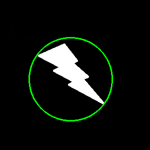

Minimum enclosing circle

9. Fitting an Ellipse

Next one is to fit an ellipse to an object. It returns the rotated rectangle in which the ellipse is inscribed:

ellipse = cv.fitEllipse(cnt)
cv.ellipse(img, ellipse, (0, 255, 0), 2)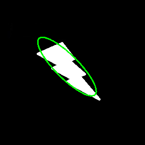

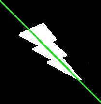
Fit ellipse

10. Fitting a Line

Similarly we can fit a line to a set of points. Below image contains a set of white points. We can approximate a straight line to it:

rows, cols = img.shape[:2]
[vx, vy, x, y] = cv.fitLine(cnt, cv.DIST_L2, 0, 0.01, 0.01)
lefty = int((-x * vy / vx) + y)
righty = int(((cols - x) * vy / vx) + y)
cv.line(img, (cols - 1, righty), (0, lefty), (0, 255, 0), 2)