Introduction to SIFT (Scale-Invariant Feature Transform)

Goal

In this chapter,

• We will learn about the concepts of SIFT algorithm
• We will learn to find SIFT Keypoints and Descriptors.

Theory

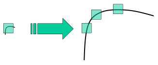
In last couple of chapters, we saw some corner detectors like Harris etc. They are rotation-invariant, which means, even if the image is rotated, we can find the same corners. But what about scaling? A corner may not be a corner if the image is scaled. For example, check a simple image below. A corner in a small image within a small window is flat when it is zoomed in the same window. So Harris corner is not scale invariant.

In 2004, D.Lowe, University of British Columbia, came up with a new algorithm, Scale Invariant Feature Transform (SIFT) in his paper, Distinctive Image Features from Scale-Invariant Keypoints, which extract keypoints and compute its descriptors.

There are mainly four steps involved in SIFT algorithm:

1. Scale-space Extrema Detection

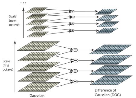
From the image above, it is obvious that we can’t use the same window to detect keypoints with different scale. For this, scale-space filtering is used. In it, Laplacian of Gaussian is found for the image with various σ values. SIFT algorithm uses Difference of Gaussians which is an approximation of LoG. Difference of Gaussian is obtained as the difference of Gaussian blurring of an image with two different σ values. This process is done for different octaves of the image in Gaussian Pyramid:

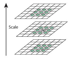
Once this DoG are found, images are searched for local extrema over scale and space. One pixel in an image is compared with its 8 neighbours as well as 9 pixels in next scale and 9 pixels in previous scales:

2. Keypoint Localization

Once potential keypoints locations are found, they have to be refined to get more accurate results. They used Taylor series expansion of scale space to get more accurate location of extrema, and if the intensity at this extrema is less than a threshold value (0.03 as per the paper), it is rejected. This eliminates any low-contrast keypoints and edge keypoints and what remains is strong interest points.

3. Orientation Assignment

Now an orientation is assigned to each keypoint to achieve invariance to image rotation. A neighbourhood is taken around the keypoint location depending on the scale, and the gradient magnitude and direction is calculated in that region.

4. Keypoint Descriptor

A 16x16 neighbourhood around the keypoint is taken. It is divided into 16 sub-blocks of 4x4 size. For each sub-block, 8 bin orientation histogram is created. So a total of 128 bin values are available. It is represented as a vector to form keypoint descriptor.

5. Keypoint Matching

Keypoints between two images are matched by identifying their nearest neighbours. If the ratio of closest-distance to second-closest distance is greater than 0.8, they are rejected. It eliminates around 90% of false matches while discards only 5% correct matches.

SIFT in OpenCV

Note that these were previously only available in the opencv contrib repo, but the patent expired in the year 2020. So they are now included in the main repo.

import numpy as np
import cv2 as cv

img = cv.imread('home.jpg')
gray = cv.cvtColor(img, cv.COLOR_BGR2GRAY)

sift = cv.SIFT_create()
kp = sift.detect(gray, None)

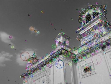
img = cv.drawKeypoints(gray, kp, img)
cv.imwrite('sift_keypoints.jpg', img)

sift.detect() function finds the keypoint in the images. Each keypoint is a special structure which has many attributes like its (x,y) coordinates, size of the meaningful neighbourhood, angle which specifies its orientation, response that specifies strength of keypoints etc.

OpenCV also provides cv.drawKeyPoints() function which draws the small circles on the locations of keypoints. If you pass a flag, cv.DRAW_MATCHES_FLAGS_DRAW_RICH_KEYPOINTS to it, it will draw a circle with size of keypoint and it will even show its orientation.

img = cv.drawKeypoints(gray, kp, img, flags=cv.DRAW_MATCHES_FLAGS_DRAW_RICH_KEYPOINTS)
cv.imwrite('sift_keypoints.jpg', img)

Now to calculate the descriptor, OpenCV provides two methods:

1. Since you already found keypoints, you can call sift.compute(): kp, des = sift.compute(gray, kp)
2. If you didn’t find keypoints, directly find keypoints and descriptors in a single step with the function, sift.detectAndCompute().

sift = cv.SIFT_create()
kp, des = sift.detectAndCompute(gray, None)

Here kp will be a list of keypoints and des is a numpy array of shape (Number of Keypoints) × 128.

Source: OpenCV Python Tutorials — Original Documentation