· Hakan Çelik · OpenCV / Image Processing · 5 dk okuma
Fourier Transform
Fourier Transform
Goals
In this section, we will learn:
- To find the Fourier Transform of images using OpenCV
- To utilize the FFT functions available in Numpy
- Some applications of Fourier Transform
- We will see following functions:
cv2.dft(),cv2.idft()
Theory
Fourier Transform is used to analyze the frequency characteristics of various filters. For images, 2D Discrete Fourier Transform (DFT) is used to find the frequency domain. A fast algorithm called Fast Fourier Transform (FFT) is used for calculation of DFT.
For a sinusoidal signal x(t) = A·sin(2πft), we can say f is the frequency of signal. You can consider an image as a signal which is sampled in two directions. So taking fourier transform in both X and Y directions gives you the frequency representation of image.
More intuitively: if the amplitude varies so fast in short time, you can say it is a high frequency signal. Where does the amplitude varies drastically in images? At the edge points, or noises. So we can say, edges and noises are high frequency contents in an image.
Fourier Transform in Numpy
np.fft.fft2() provides us the frequency transform which will be a complex array. The zero frequency component (DC component) will be at top-left corner. Use np.fft.fftshift() to bring it to center:
import cv2 as cv
import numpy as np
from matplotlib import pyplot as plt
img = cv.imread('messi5.jpg', cv.IMREAD_GRAYSCALE)
assert img is not None, "file could not be read, check with os.path.exists()"
f = np.fft.fft2(img)
fshift = np.fft.fftshift(f)
magnitude_spectrum = 20 * np.log(np.abs(fshift))
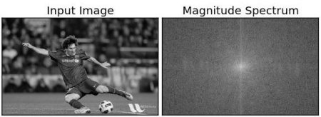
plt.subplot(121), plt.imshow(img, cmap='gray')
plt.title('Input Image'), plt.xticks([]), plt.yticks([])
plt.subplot(122), plt.imshow(magnitude_spectrum, cmap='gray')
plt.title('Magnitude Spectrum'), plt.xticks([]), plt.yticks([])
plt.show()Result look like below:
You can see more whiter region at the center showing low frequency content is more.
Now you can do some operations in frequency domain, like high pass filtering and reconstruct the image. Remove the low frequencies by masking with a rectangular window of size 60x60, then apply inverse shift using np.fft.ifftshift() so that DC component again comes at the top-left corner:
rows, cols = img.shape
crow, ccol = rows // 2, cols // 2
fshift[crow-30:crow+31, ccol-30:ccol+31] = 0
f_ishift = np.fft.ifftshift(fshift)
img_back = np.fft.ifft2(f_ishift)
img_back = np.real(img_back)

plt.subplot(131), plt.imshow(img, cmap='gray')
plt.title('Input Image'), plt.xticks([]), plt.yticks([])
plt.subplot(132), plt.imshow(img_back, cmap='gray')
plt.title('Image after HPF'), plt.xticks([]), plt.yticks([])
plt.subplot(133), plt.imshow(img_back)
plt.title('Result in JET'), plt.xticks([]), plt.yticks([])
plt.show()
Result look like below:
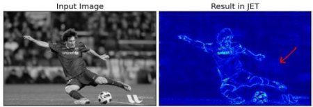
The result shows High Pass Filtering is an edge detection operation. You can also see some artifacts called ringing effects caused by the rectangular window. Better option is Gaussian Windows.
Fourier Transform in OpenCV
OpenCV provides cv2.dft() and cv2.idft() for this. The input image should be converted to np.float32 first:
import numpy as np
import cv2 as cv
from matplotlib import pyplot as plt

img = cv.imread('messi5.jpg', cv.IMREAD_GRAYSCALE)
assert img is not None, "file could not be read, check with os.path.exists()"

dft = cv.dft(np.float32(img), flags=cv.DFT_COMPLEX_OUTPUT)
dft_shift = np.fft.fftshift(dft)

magnitude_spectrum = 20 * np.log(cv.magnitude(dft_shift[:, :, 0], dft_shift[:, :, 1]))

plt.subplot(121), plt.imshow(img, cmap='gray')
plt.title('Input Image'), plt.xticks([]), plt.yticks([])
plt.subplot(122), plt.imshow(magnitude_spectrum, cmap='gray')
plt.title('Magnitude Spectrum'), plt.xticks([]), plt.yticks([])
plt.show()
Note: You can also use
cv2.cartToPolar()which returns both magnitude and phase in a single shot.
Now apply LPF (Low Pass Filter) to remove high frequency contents — this blurs the image. Create a mask with high value (1) at low frequencies:
rows, cols = img.shape
crow, ccol = rows // 2, cols // 2
# create a mask first, center square is 1, remaining all zeros
mask = np.zeros((rows, cols, 2), np.uint8)
mask[crow-30:crow+30, ccol-30:ccol+30] = 1
# apply mask and inverse DFT
fshift = dft_shift * mask
f_ishift = np.fft.ifftshift(fshift)
img_back = cv.idft(f_ishift)
img_back = cv.magnitude(img_back[:, :, 0], img_back[:, :, 1])
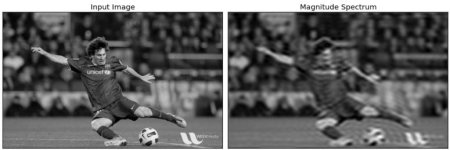
plt.subplot(121), plt.imshow(img, cmap='gray')
plt.title('Input Image'), plt.xticks([]), plt.yticks([])
plt.subplot(122), plt.imshow(img_back, cmap='gray')
plt.title('Magnitude Spectrum'), plt.xticks([]), plt.yticks([])
plt.show()See the result:
Note: OpenCV functions
cv2.dft()andcv2.idft()are faster than Numpy counterparts. But Numpy functions are more user-friendly.
Performance Optimization of DFT
Performance of DFT calculation is best for array sizes that are power of two. OpenCV provides cv2.getOptimalDFTSize() for this:
img = cv.imread('messi5.jpg', cv.IMREAD_GRAYSCALE)
rows, cols = img.shape
print("{} {}".format(rows, cols))     # 342 548

nrows = cv.getOptimalDFTSize(rows)
ncols = cv.getOptimalDFTSize(cols)
print("{} {}".format(nrows, ncols))   # 360 576
Then pad with zeros using cv2.copyMakeBorder():
right = ncols - cols
bottom = nrows - rows
nimg = cv.copyMakeBorder(img, 0, bottom, 0, right, cv.BORDER_CONSTANT, value=0)
This shows about 4x speedup. OpenCV functions are also around 3x faster than Numpy functions.
Why Laplacian is a High Pass Filter?
Take the Fourier transform of different filter kernels and analyze their frequency responses:
import cv2 as cv
import numpy as np
from matplotlib import pyplot as plt

mean_filter = np.ones((3, 3))
x = cv.getGaussianKernel(5, 10)
gaussian = x * x.T
scharr = np.array([[-3, 0, 3], [-10, 0, 10], [-3, 0, 3]])
sobel_x = np.array([[-1, 0, 1], [-2, 0, 2], [-1, 0, 1]])
sobel_y = np.array([[-1, -2, -1], [0, 0, 0], [1, 2, 1]])
laplacian = np.array([[0, 1, 0], [1, -4, 1], [0, 1, 0]])

filters = [mean_filter, gaussian, laplacian, sobel_x, sobel_y, scharr]
filter_name = ['mean_filter', 'gaussian', 'laplacian', 'sobel_x', 'sobel_y', 'scharr_x']
fft_filters = [np.fft.fft2(x) for x in filters]
fft_shift = [np.fft.fftshift(y) for y in fft_filters]
mag_spectrum = [np.log(np.abs(z) + 1) for z in fft_shift]

for i in range(6):
    plt.subplot(2, 3, i + 1), plt.imshow(mag_spectrum[i], cmap='gray')
    plt.title(filter_name[i]), plt.xticks([]), plt.yticks([])
plt.show()
See the result:
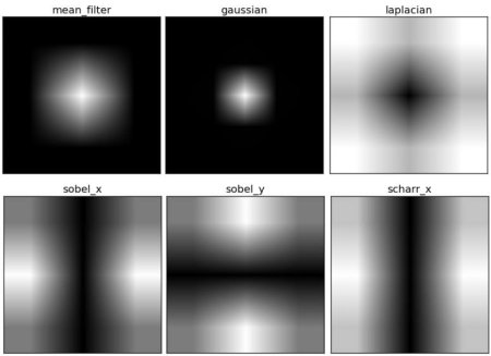
From image, you can see what frequency region each kernel blocks, and what region it passes.
Additional Resources
- An Intuitive Explanation of Fourier Theory by Steven Lehar
- Fourier Transform at HIPR
- What does frequency domain denote in case of images?